Science Archives

Writing in Secondary Schools – understanding and applying grammar in context

Overview

The focus of this three-day course presented by Kathy Rushton and Joanne Rossbridge is supporting participants to identify the language demands of texts commonly read and written in the secondary school and recognising the features of their students’ writing.

We will focus on the teaching of writing as the context in which grammar is taught to support meaning and we will outline those grammatical features which best support teachers to make an impact on students who are writing extended responses.

Our aim is not to focus on the basics, but we will briefly review or address grammar for those who may be addressing it explicitly for the first time. This will support participants to identify and address their students’ needs as they analyse their written work. We will provide practical examples of strategies for engaging students in writing and supporting students to write effectively.

Sydney

Day 1 – Friday 9 May 2025

Day 2 – Friday 23 May 2025

Day 3 – Friday 13 June 2025

Federation House

23-33 Mary St, Surry Hills, NSW 2010

Day 1 – Language and Literacy

Talking and Listening – What’s the difference? (Grammatical intricacy and lexical density)

Reading – What’s going on? (The verbal group)

Overview of sessions.
Discussion of Assessment tasks.
Introduction of field, tenor and mode:

Mode continuum.
Types of verbs and aspects of verbal groups identified and discussed.
The importance of teacher identification of verbal groups for exploring clause patterns in texts students are both reading and writing.

Whole group trials and share strategies for supporting students to explore verbal groups

Day 2 – Language Choices

Theme (Marked)

Reading – Who and What? (The noun group)

Writing – Where? When? How? (Adverbials and Theme)

Aspects of the extended noun group explained as well as the use of noun groups in developing lexically dense texts.
Analysis of texts suitable for all stages. Discussion at clause and group levels building on knowledge of the verb group to introduce the concept of marked theme of clause realised as an adverbial phrase of time, place or manner.
Analysis of texts and strategies for teaching adverbial phrases and their use in thematic position across the stages of texts.
Sharing of scaffolds.

Day 3 – Creating Cohesive texts

Sentence structure

The third voice in your classroom – Using quality texts. (Nominalisation)

Identifying the role of nominalisation and active and passive voice in quality texts and how they are used to develop theme across the stages of texts.
Identifying strategies for developing writing through a joint construction.
Sharing of notes for a joint construction.

Please note each day is accredited separately

Day 1 Accreditation

Completing Writing in Secondary Schools – understanding and applying grammar in context (Language and Literacy) will contribute 5 hours of NSW Education Standards Authority (NESA) Accredited PD in the priority area of Delivery and Assessment of NSW Curriculum/EYLF addressing Standard Descriptor(s) 2.5.2 and 3.5.2 from the Australian Professional Standards for Teachers towards maintaining Proficient Teacher Accreditation in NSW.

Day 2 Accreditation

Completing Writing in Secondary Schools – understanding and applying grammar in context (Language choices) will contribute 5 hours of NSW Education Standards Authority (NESA) Accredited PD in the priority area of Delivery and Assessment of NSW Curriculum/EYLF addressing Standard Descriptor(s) 2.5.2 and 3.3.2 from the Australian Professional Standards for Teachers towards maintaining Proficient Teacher Accreditation in NSW.

Day 3 Accreditation

Completing Writing in Secondary Schools – understanding and applying grammar in context (creating cohesive texts) will contribute 5 hours of NSW Education Standards Authority (NESA) Accredited PD in the priority area of Delivery and Assessment of NSW Curriculum/EYLF addressing Standard Descriptor(s) 2.5.2, 3.3.2 from the Australian Professional Standards for Teachers towards maintaining Proficient Teacher Accreditation in NSW.

“The course delivered by Jo and Kathy has been nothing short of positive and eye-opening. As a science teacher, I struggled to find why it is my role to teach literacy but that was only out of fear as I didn’t have much knowledge on language. This course not only expanded my knowledge but bolstered my confidence in implementing new strategies in the classroom. The course provided a clear understanding of literacy, allowing me to see the connections and applications of these concepts in a way that can resonate with my students. The experience I had implementing a joint construction has led to a boost in my self-efficacy. Overall, the professional learning course has been beneficial for me. It has provided me with tools and resources to enhance my teaching and better support my students on their learning journey. Thank you for the opportunity and experience.”

“Best PL I have done.”

“Presenters were highly engaging, approachable and demonstrated exceptional knowledge and pedagogical practice.”

“This course was extremely interesting and gave me many ideas for my own teaching – and my own learning.”

“This course was fantastic! Essential learning for all teachers! Thank you!”

“Thank you for the amazing and useful sessions! I feel more confident about grammar now.’

“I enjoyed the structure and engaging with colleagues regarding the strategies we started implementing into our classes.”

Kathy Rushton

Kathy Rushton is interested in the development of language and literacy especially in disadvantaged communities. She has worked as a classroom teacher and literacy consultant and provides professional learning for teachers in the areas of language and literacy development. Her current research projects include a study of multilingual pre-service teachers and the impact that teacher professional learning has on the development of a creative pedagogical stance which supports translanguaging and student identity and wellbeing.

Joanne Rossbridge

Joanne Rossbridge is an independent language and literacy consultant working in both primary and secondary schools and with teachers across Australia. She has worked as a classroom teacher and literacy consultant with the DET (NSW). Her expertise and much of her experience is in working with students from diverse linguistic and cultural backgrounds. Joanne is particularly interested in student and teacher talk and how talk about language can assist the development of language and literacy.

Secondary teachers especially teachers of all subjects requiring extended response writing such as HSIE, English, PDHPE and Science.

Teacher Librarians

$660 for three days

Three whole-day workshops with participants actively engaged in each session and undertaking pre-course and in-between course readings.

JPL Articles

Helping Your Students to Become Better Writers

Critical Literacy in English and History: Stages 3 & 4

Helping Your Students to Become Better Writers

Joanne Rossbridge & Kathy Rushton share a framework for improved extended response writing…

Introduction

Teacher knowledge about language and how it works is critical for not only developing dialogue around texts but can make explicit for students the strategies used by effective writers across subject areas. This requires understanding of the grammatical features of the common genres students commonly are asked to write in the secondary school.

This article looks at the extended response to support teachers to analyse student writing and examine both the language and literacy demands related to writing extended responses in secondary settings. The following outlines the approach and principles that are drawn upon in both a one-day and three-day CPL course entitled Conversations about Text in the Secondary School and Developing Dialogue about Text in the Secondary Schools respectively.

Making appropriate choices – Field, Tenor and Mode Framework for writing

Texts can be discussed using a framework developed by Michael Halliday (Halliday & Hasan, 1985) in which the three critical aspects of the register of the text, field, tenor and mode are utilised to analyse and understand how successful texts are constructed to reflect their context and purpose:

Field refers to the subject matter of the text and this of course will differ across and within subjects;
Tenor is the relationship established between the reader and writer;
Mode addresses the nature of the text itself and the role language plays within it.

When viewed together, all students can be supported to understand the range of language choices which need to be made to successfully realise the purpose of a text for the audience it is addressing.

For further explanation see Halliday & Hasan, 1985 and Rossbridge & Rushton, 2015.

This helps students to realise that careful reading and note-taking may address field but to meet the challenges of engaging an audience and establishing a clear purpose for their text a range of other language choices need to be made.

The following framework provides teachers with a time-saving and focussed way to provide the support that developing writers may need at all levels of text from word, clause, group and sentence to paragraph and text levels (Derewianka, 2011).

Choices in context: a case study from the ancients

The context for writing in secondary schools is provided by the subject areas. Students may be involved in field building through the focus on teaching content around a topic such as an example of The Ancient World in History. In addition to acquiring the field knowledge we also need to be explicit about who the audience may be that they are writing for as well as the relationship between the writer and reader.

The following examples show how the field of the writing may be similar but the tenor and mode differ. This can be seen by the more personal connection with the audience in Text 1 while Text 2 seems to convey more authority on the topic. In addition, the mode of the texts may differ in that the writing may be more spoken or written-like as evident in Text 2, which sounds more written-like or academic in the way the ideas have been packaged and organised.

Text 1

Have you ever wondered what life was like for women in Ancient Sparta? They had lots of power and could think for themselves more than some of the other women in other places in Greece.

Text 2

Spartan women had a reputation for strength and independence. They enjoyed greater freedom and power than women in other city-states in Ancient Greece.

This framework for considering and talking about language choices in context can provide the basis of a strong scaffold (Hammond, 2001; Vygotsky, 1986) for adolescent writers.

Writing pedagogy

The genre based pedagogy known as the Teaching Learning Cycle was originally developed by Sydney School genre theorists… [it] has proved a powerful resource for scaffolding literacy development, with numerous published units of work documenting and/or guiding its implementation. (Humphrey & Macnaught, 2011, p. 99)

The Teaching Learning Cycle includes building the field, text deconstruction, joint construction and independent construction. Our focus is on supporting teachers to undertake the more challenging text deconstruction and joint construction.

We consider that the critical dialogue about text occurs during text deconstruction and joint construction (Rossbridge & Rushton, 2014). In many classrooms, texts are modelled but the rich language about language, metalanguage, can only be developed when the teacher and students talk together about the language features of the texts they are reading or writing (Lemke, 1989).

For this reason, one of the courses involves the conversations about text that teachers can develop to support writing development (Rossbridge & Rushton, 2010 & 2011). By using the field, tenor, mode framework for writing, not just the field (content) but also the tenor (relationship) and mode (nature) can easily be the focus of these conversations.

What a conversation might lead to

The following transcript provides an example of the conversations which might occur between a teacher and students. In this example from a whole class joint construction the notion of perspective in History texts is explored by considering the development of the noun group to name participants in events.

Student: Dan would say he’s like a visitor because he wouldn’t say he is trespassing or doing anything wrong. He’d say he’s visiting and helping out his country.

Student: You probably know that their settling there as a new country.

Teacher: So are you saying he’s a settler?

Student: Yeah. Like saying he would know he’s not really going to be going anywhere.

Teacher: So, is he a visitor or a settler?

Students: Settler.

Teacher: What have we built? Dan, who was a young British settler. What have we just built?

Student: Noun group.

Teacher: Yes, we’ve built a whole noun group with an adjectival clause.

(See Rossbridge & Rushton, 2014 & 2015)

Key principles for developing a critical dialogue about text

The key principles for developing the critical dialogue about text are, in our view, language, the learner and the support or scaffold provided for the student. The teacher needs to be very clear about the language needed to write target texts as well as having a clear view of the purpose of talk in the classroom.
The dialogue can be supported by questioning, Think Alouds (when the teacher verbalises their thinking as they read for meaning to model the thinking skills required for comprehension) and other strategies which provide opportunities for talk and substantive communication.
The learner needs to be both engaged and supported to undertake risks (Hammond, 2001) if they are to master the challenges of writing an extended response in an academic context. The support needed is not just modelling but the ability to hand over the tasks to the students (Gibbons, 2002 & 2006) at the right point, the Zone of Proximal Development (ZPD) (Hammond, 2001; Vygotsky, 1986). This may require both micro and macro scaffolding when programming and teaching.
One of the most important understandings about language development is that it can be viewed on a continuum from spoken-like to written-like language, the mode continuum. At one end of the continuum is oral language which differs from written language mainly in its density. Written language is lexically dense in the sense that more meaning is carried in fewer words (Halliday, 1985). The challenge teachers face is to support students to develop the lexically dense texts which are valued in our education system.Written language is lexically dense in the sense that more meaning is carried in fewer words

Nominalisation and theme

Using the framework of field, tenor and mode two very useful tools for writing can be drawn upon. These are the features of nominalisation and theme which can be identified in texts. Students can be taught how to use them to make their texts more effective. Nominalisation is a resource that allows writers to change verbs, conjunctions and adjectives into nouns.

Making language more powerful

We should reduce mining near the coastline.

The reduction of mining near the coastline will result in greater preservation of coastal ecosystems.

In the example the verb group in the first clause has been turned into a noun group (nominalised) and placed at the front of the second clause in theme position. By doing this the main focus of the writing can be put up front, the writing sounds more written-like and by repackaging the first clause into a noun group the writer is able to add additional information.

Such conversation and dialogue around text enables students to take on knowledge about language in the context of texts and apply it to their own writing.

The use of these features relates to the genre of the target text (Macken & Slade, 1993; Martin & White, 2005; Martin & Rose, 2008). While unfamiliarity may initially challenge students, when teachers become adept at deconstructing both modelled and student texts even very young students are able to grasp the concepts and begin to utilise them in their writing.

Our CPL courses demonstrate a range of strategies for developing extended responses which include the effective use of these features and support students to master them.

References:

Derewianka, B. (2011) A new grammar companion for primary teachers. Newtown: PETAA

Gibbons, P. (2006) Bridging discourses in the ESL classroom: Students, teachers and researchers (pp.59-70). London: Continuum

Gibbons, P. (2002) Scaffolding language, scaffolding learning: Teaching second language learners in the mainstream classroom (pp.77-101). Portsmouth: Heinemann:

Halliday, M.A.K.(1985) Spoken and written language (pp.61-67). Victoria: Deakin University Press

Halliday, M.A.K. & Hasan, R. (1976) Cohesion in English (pp.238-245). London: Longman

Halliday, M.A.K. & Hasan, R. (1985) Language, context, and text: Aspects of language in a social-semiotic perspective (pp.238-245). Victoria: Deakin University Press

Hammond, J. (Ed.) (2001) What is scaffolding? Scaffolding teaching and learning in language and literacy education (pp.1-14). Newtown:PETAA

Humphrey S., Droga, L. & Feez, S. (2012) Grammar and meaning: New Edition. Newtown: PETAA

Humphrey, S. & Macnaught S. (2011) Revisiting joint construction in the tertiary context. Australian Journal of Language and Literacy. 34(1), 98-116

Lemke, J. (1989) Making text talk: Theory into practice. Columbus, Ohio: College of Education Ohio State University

Macken, M. & Slade, D. (1993) Assessment: A foundation for effective learning in the school context. In Cope. B & Kalantzis, M. (1993) The powers of literacy: A genre approach to teaching writing. (pp.203-222) Bristol, P.A.: The Falmer Press

Martin, J. & Rose, D. (2008) Genre relations: Mapping culture London: Equinox Publishing

Martin, J. & White, R. (2005) The language of evaluation: Appraisal in English. (pp.26-38) Basingstoke: Palgrave Macmillan

Rossbridge, J. & Rushton, K. (2015) Put it in writing. Newtown: PETAA

Rossbridge, J. & Rushton, K. (2014) PETAA Paper 196 The critical conversation about text: Joint construction. Newtown: PETAA http://www.petaa.edu.au/imis_prod/w/Teaching_Resources/PETAA_Papers/w/Teaching_Resources/PPs/PETAA_Paper_196___The_critical_conversation_.aspx

Rossbridge, J. & Rushton, K. (2010) Conversations about text: Teaching grammar with literary texts. Newtown: PETAA

Rossbridge, J. & Rushton, K. (2011) Conversations about text: Teaching grammar with factual texts. Newtown: PETAA

Vygotsky, L. (1986) Thought and Language. Cambridge, Massachusetts: MIT Press pp.xi-xliii

About the authors

Dr Kathy Rushton is interested in the development of literacy, especially in socio-economically disadvantaged communities with students learning English as an additional language or dialect. She has worked as a literacy consultant, EAL/D and classroom teacher with the DOE (NSW), and in a range of other educational institutions. Kathy is a lecturer in the Faculty of Education and Social Work at the University of Sydney.

Joanne Rossbridge is an independent English, language, literacy and EAL/D consultant working in both primary and secondary schools across Sydney and Australia. She has worked as a classroom and ESL teacher, literacy consultant and lecturer in universities. Much of her experience has involved working with students with language backgrounds other than English. Joanne is particularly interested in student and teacher talk and how talk about language can assist in the development of language and literacy skills.

Uncertainty, Error and Confidence in Data

Jim Sturgiss provides a straightforward guide to teaching some scientific concepts that are now part of the new Science syllabuses…

Uncertainty is a statistical concept found in the Assessing data and information outcome of the new Science syllabuses:.

WS 5.2 assess error, uncertainty and limitations in data (ACSBL004, ACSBL005, ACSBL033, ACSBL099)
This concept is not found in the previous syllabuses.
This paper addresses uncertainty as a means of describing the accuracy of a series of measurements or as a means of comparing two sets of data. Uncertainty, or confidence, is described in terms of mean and standard deviation of a dataset. Standard deviation is a concept encountered by students in Stage 5.3 Mathematics and Stage 6 Standard 2 Mathematics.
Not explored in this paper is the use of Microsoft Excel or Google Sheets which can calculate uncertainty of datasets with ease (=STDEV.S(number1, number2,…).

Figure 1 Karl Pearson

Karl Pearson (Figure 1), the great 19th-century biostatistician and eugenist, first described mathematical methods for determining the probability distributions of scientific measurements, and these methods form the basis of statistical applications in scientific research. Statistical techniques allow us to estimate uncertainty and report the error surrounding a value after repeated measurement of that value.

1. Accuracy, Precision and Error

Accuracy is how close a measurement is to the correct value for that measurement. The precision of a measurement system refers to how close the agreement is between repeated measurements (which are repeated under the same conditions). Measurements can be both accurate and precise, accurate but not precise, precise but not accurate, or neither.

Precision and Imprecision

Precision (see Figure 2) refers to how well measurements agree with each other in multiple tests. Random error, or Imprecision, is usually quantified by calculating the coefficient of variation from the results of a set of duplicate measurements.

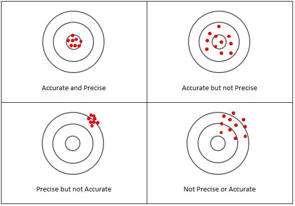
Figure 2 Accuracy and precision

The accuracy of a measurement is how close a result comes to the true value.

Error

When randomness is attributed to errors, they are “errors” in the sense in which that term is used in statistics.

Systematic error (bias) occurs with the same value, when we use the instrument in the same way (eg calibration error) and in the same case. This is sometimes called statistical bias.

It may often be reduced with standardized procedures. Part of the learning process in the various sciences is learning how to use standard instruments and protocols so as to minimize systematic error.

Random error, which may vary from one observation to another. Random error (or random variation) is due to factors which cannot, or will not, be controlled. Random error often occurs when instruments are pushed to the extremes of their operating limits. For example, it is common for digital balances to exhibit random error in their least significant digit. Three measurements of a single object might read something like 0.9111g, 0.9110g, and 0.9112g.

Systematic error or Inaccuracy (see Figure 3) is quantified by the average difference (bias) between a set of measurements obtained with the test method with a reference value or values obtained with a reference method.

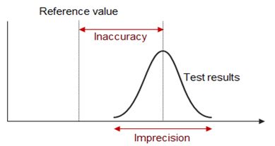
Figure 3 Imprecision and in accuracy

2. Uncertainty

There is uncertainty in all scientific data. Uncertainty is reported in terms of confidence.

Uncertainty is the quantitative estimation of error present in data; all measurements contain some uncertainty generated through systematic error and/or random error.
Acknowledging the uncertainty of data is an important component of reporting the results of scientific investigation.
Careful methodology can reduce uncertainty by correcting for systematic error and minimizing random error. However, uncertainty can never be reduced to zero.

Estimating the Experimental Uncertainty For a Single Measurement

Any measurement made will have some uncertainty associated with it, no matter the precision of the measuring tool. So how is this uncertainty determined and reported?

The uncertainty of a single measurement is limited by the precision and accuracy of the measuring instrument, along with any other factors that might affect the ability of the experimenter to make the measurement.

For example, if you are trying to use a ruler to measure the diameter of a tennis ball, the uncertainty might be ± 5 mm, but if you used a Vernier caliper, the uncertainty could be reduced to maybe ± 2 mm. The limiting factor with the ruler is parallax, while the second case is limited by ambiguity in the definition of the tennis ball’s diameter (it’s fuzzy!). In both of these cases, the uncertainty is greater than the smallest divisions marked on the measuring tool (likely 1 mm and 0.05 mm respectively).

Unfortunately, there is no general rule for determining the uncertainty in all measurements. The experimenter is the one who can best evaluate and quantify the uncertainty of a measurement based on all the possible factors that affect the result. Therefore, the person making the measurement has the obligation to make the best judgment possible and to report the uncertainty in a way that clearly explains what the uncertainty represents:

Measurement = (measured value ± standard uncertainty) unit of measurement.
For example, where the ± standard uncertainty indicates approximately a 68% confidence interval, the diameter of the tennis ball may be written as 6.7 ± 0.2 cm.
Alternatively, where the ± standard uncertainty indicates approximately a 95% confidence interval, the diameter of the tennis ball may be written as 6.7 ± 0.4 cm.

Estimating the Experimental Uncertainty For a Repeated Measure (Standard Deviation).

Suppose you time the period of oscillation of a pendulum using a digital instrument (that you assume is measuring accurately) and find: T = 0.44 seconds. This single measurement of the period suggests a precision of ±0.005 s, but this instrument precision may not give a complete sense of the uncertainty. If you repeat the measurement several times and examine the variation among the measured values, you can get a better idea of the uncertainty in the period.

For example, here are the results of 5 measurements, in seconds: 0.46, 0.44, 0.45, 0.44, 0.41.

For this situation, the best estimate of the period is the average, or mean.

Whenever possible, repeat a measurement several times and average the results. This average is generally the best estimate of the “true” value (unless the data set is skewed by one or more outliers). These outliers should be examined to determine if they are bad data points, which should be omitted from the average, or valid measurements that require further investigation.

Generally, the more repetitions you make of a measurement, the better this estimate will be, but be careful to avoid wasting time taking more measurements than is necessary for the precision required.

Consider, as another example, the measurement of the thickness of a piece of paper using a micrometer. The thickness of the paper is measured at a number of points on the sheet, and the values obtained are entered in a data table.

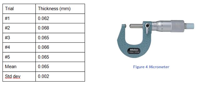
This average is the best available estimate of the thickness of the piece of paper, but it is certainly not exact. We would have to average an infinite number of measurements to approach the true mean value, and even then, we are not guaranteed that the mean value is accurate because there is still some systematic error from the measuring tool, which can never be calibrated perfectly. So how do we express the uncertainty in our average value?

The most common way to describe the spread or uncertainty of the data is the standard deviation

Figure 5 Standard deviations of a normal distribution

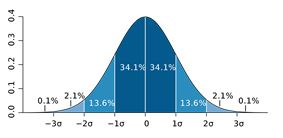
The significance of the standard deviation is this:

if you now make one more measurement using the same micrometer, you can reasonably expect (with about 68% confidence) that the new measurement will be within 0.002 mm of the estimated average of 0.065 mm. In fact, it is reasonable to use the standard deviation as the uncertainty associated with this single new measurement.

This is written:
The thickness of 80 gsm paper (n=5) averaged 0.065 (s = 0.002mm)
s = standard deviation
OR
The thickness of 80 gsm paper (n=5) averaged 0.065 ± 0.004 mm to a 95% confidence level.
(0.004 mm represents 2 standard deviations, 2s)

Standard Deviation of the Means (Standard Error of Mean (SEM))

The standard error is a measure of the accuracy of the estimate of the mean from the true or reference value. The main use of the standard error of the mean is to give confidence intervals around the estimated means for normally distributed data, not for the data itself but for the mean.

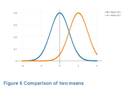
If measured values are averaged, then the mean measurement value has a much smaller uncertainty, equal to the standard error of the mean, which is the standard deviation divided by the square root of the number of measurements.

Standard error is often us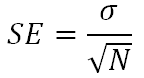ed to test (in terms of null hypothesis testing) differences between means.

For example, two populations of salmon fed on two different diets may be considered significantly different if the 95% confidence intervals (two std errors) around the estimated fish sizes under Diet A do not cross the estimated mean fish size under Diet B.

Note that the standard error of the mean depends on the sample size, as the standard error of the mean shrinks to 0 as sample size increases to infinity.

Figure 7 Salmon

Standard Error of Mean (SEM) Versus Standard Deviation

In scientific and technical literature, experimental data are often summarized either using the mean and standard deviation of the sample data or the mean with the standard error. This often leads to confusion about their interchangeability. However, the mean and standard deviation are descriptive statistics, whereas the standard error of the mean is descriptive of the random sampling process.

The standard deviation of the sample data is a description of the variation in measurements, whereas, the standard error of the mean is a probabilistic statement about how the sample size will provide a better bound on estimates of the population mean, in light of the central limit theorem.

Put simply, the standard error of the sample mean is an estimate of how far the sample mean is likely to be from the population mean, whereas the standard deviation of the sample is the degree to which individuals within the sample differ from the sample mean. If the population standard deviation is finite, the standard error of the mean of the sample will tend to zero with increasing sample size. This is because the estimate of the population mean will improve, while the standard deviation of the sample will tend to approximate the population standard deviation as the sample size increases.

Confidence Levels

The confidence level represents the frequency (i.e. the proportion) of possible confidence intervals that contain the true value of the unknown population parameter. Most commonly, the 95.4% (“two sigma”) confidence level is used. However, other confidence levels can be used, for example, 68.3% (“one sigma”) and 99.7% (“three sigma”).

Conclusion

Knowledge of normally distributed data and standard deviation are key to understanding the notions of statistical uncercertainty and confidence. These concepts are extended to the standard error of mean so that the significance of differences between two related datasets can be determined.

Glossary

Absolute error The absolute error of a measurement is half of the smallest unit on the measuring device. The smallest unit is called the precision of the device.

Array An array is an ordered collection of objects or numbers arranged in rows and columns.

Bias This generally refers to a systematic favouring of certain outcomes more than others, due to unfair influence (knowingly or otherwise).

Confidence level The probability that the value of a parameter falls within a specified range of values. For example 2s = 95% confidence level.

Data cleansing Detecting and removing errors and inconsistencies from data in order to improve the quality of data (also known as data scrubbing).

Data set An organised collection of data.

Descriptive statistics These are statistics that quantitatively describe or summarise features of a collection of information.

Large data sets Data sets that must be of a size to be statistically reliable and require computational analysis to reveal patterns, trends and associations.

Limits of accuracy The limits of accuracy for a recorded measurement are the possible upper and lower bounds for the actual measurement.

Measures of central tendency Measures of central tendency are the values about which the set of data values for a particular variable are scattered. They are a measure of the centre or location of the data. The two most common measures of central tendency are the mean and the median.

Measures of spread Measures of spread describe how similar or varied the set of data values are for a particular variable. Common measures of spread include the range, combinations of quantiles (deciles, quartiles, percentiles), the interquartile range, variance and standard deviation.

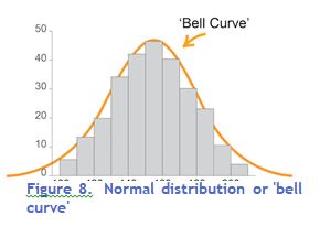Normal distribution The normal distribution is a type of continuous distribution whose graph looks like this:

The mean, median and mode are equal and the scores are symmetrically arranged either side of the mean.

The graph of a normal distribution is often called a ‘bell curve’ due to its shape.

Reliability An extent to which repeated observations and/or measurements taken under identical circumstances will yield similar results.

Sampling This is the selection of a subset of data from a statistical population. Methods of sampling include:

systematic sampling – sample data is selected from a random starting point, using a fixed periodic interval
self-selecting sampling – non-probability sampling where individuals volunteer themselves to be part of a sample
simple random sampling – sample data is chosen at random; each member has an equal probability of being chosen
stratified sampling – after dividing the population into separate groups or strata, a random sample is then taken from each group/strata in an equivalent proportion to the size of that group/strata in the population
A sample can be used to estimate the characteristics of the statistical population.

Standard deviation This is a measure of the spread of a data set. It gives an indication of how far, on average, individual data values are spread from the mean.

Standard error The standard error of the mean (SEM) is the standard deviation of the sampling distribution of the mean.

Uncertainty Any single value has an uncertainty equal to the standard deviation. However, if the

values are averaged, then the mean measurement value has a much smaller uncertainty, equal to the standard error of the mean, which is the standard deviation divided by the square root of the number of measurements.

Works Cited

Measurements and Error Analysis, www.webassign.net/question_assets/unccolphysmechl1/measurements/manual.html.

Altman, Douglas G, and J Martin Bland. “Standard Deviations and Standard Errors.” BMJ (Clinical Research Ed.), BMJ Publishing Group Ltd., 15 Oct. 2005, www.ncbi.nlm.nih.gov/pmc/articles/PMC1255808/.

Hertzog, Lionel. “Standard Deviation vs Standard Error.” DataScience , 28 Apr. 2017, https://datascienceplus.com/standard-deviation-vs-standard-error/

Mott, Vallerie. “Introduction to Chemistry.”
https://courses.lumenlearning.com/introchem/chapter/accuracy-precision-and-error/

Schoonjans, Frank. “Definition of Accuracy and Precision.” MedCalc, MedCalc Software, 9 Nov. 2018, www.medcalc.org/manual/accuracy_precision.php.

“Standard Error.” Wikipedia, Wikimedia Foundation, 7 Mar. 2019,
https://en.wikipedia.org/wiki/Standard_error

2336 | NSW Education Standards,
https://educationstandards.nsw.edu.au/wps/portal/nesa/11-12/stage-6-learning-areas/stage-6-science/biology-2017/content/2336

1319 | NSW Education Standards, https://educationstandards.nsw.edu.au/wps/portal/nesa/11-12/stage-6-learning-areas/stage-6-mathematics/mathematics-standard-2017/content/1319

Jim is an educational researcher and independent educational consultant. His M.Ed (Hons) thesis used an experimental design to evaluate the effectiveness of a literacy and learning program (1997). A recipient of the NSW Professional Teaching Council’s Distinguished Service Award for leadership in delivering targeted professional learning to teachers, he works with schools to align assessment, reporting and learning practice. He has been a head teacher of Science in two large Sydney high schools, as well as HSC Chemistry Senior Marker and Judge. For many years he served as a DoE Senior Assessment Advisor where he developed many statewide assessments, (ESSA, SNAP, ELLA, BST) and as Coordinator: Analytics where he developed reports to schools for statewide assessments and NAPLAN. He is a contributing author to the new Pearson Chemistry for NSW and to Macquarie University’s HSC Study Lab for Physics.

Building Confidence and Success in Stage 6

Khya Brooks suggests an approach to the HSC which can reduce everyone’s anxiety…

On the day my first HSC classes’ results were released, I was nervous and excited. However, I did not expect the reactions that I witnessed.

Many people turned to me and said “Congratulations. You did so well”, as though I had just sat the tests myself. Meanwhile, some of my colleagues were sitting with their head in their hands saying “I didn’t even get one band 6. What happened?” The rest of the day was spent listening to colleagues criticise their own practice and try to justify their classes’ outcomes to themselves; “Oh, I should have focused more on this area in the syllabus…” and “If only I had thought to revise this case study more thoroughly”.

What I learnt that day was to internalise the HSC results as though they were my own. I learned that my classes’ success somehow translated into how valuable I was as a teacher. The day was not spent celebrating, it was spent critically reflecting. Sure, this is great practice for long-term improvement, but what I have found is that it has also increased the pressure experienced by teachers. I have noticed that this pressure is then often transferred onto students, resulting in unnecessarily increased anxiety throughout the school.

I argue that this approach is reflective of a growing individualistic and negative culture within society and therefore teaching; which positions individual teachers rather than school systems or society more widely as solely responsible for student outcomes. This anxiety is reinforced by constant questions from the school executive, such as “Did you differentiate enough?”, “Are you providing enough scaffolds?”, “How many band 6s will you get this year?”

There is often too much pressure on many of the adults and, subsequently, many of the children at school.

I thought school was supposed to be joyful!

What to do?

So, I decided to actively address this cultural shift. I wanted students to own their own learning, rather than assuming it was all my responsibility. I began to reshape my programs, assessments and my overall practice. The more confident and successful my students became with their skills, the more confident and successful I felt within my practice. Our collective anxiety melted away and school days became more positive.

I found this new approach enabled me to have a better range of measures to gauge my success as a teacher. Rather than relying on quantitative numbers at the end of the HSC, I established a clearer set of procedures that allowed me, and the students themselves, to better measure our progress.

Below are some practical strategies that have helped me in achieving this cultural shift in my classroom, with a view to empower learners and improve their confidence, and ultimately, their success. I will focus prominently on the strategies utilised with my Society and Culture classes, but they are strategies that are easily transferrable to other subjects.

Please note, I work in a partially-selective public school in South-West Sydney. This means I have a large range of students; from high to lower ability, from advantaged to disadvantaged backgrounds, and from the disengaged through to some ‘over workers’. I have found that these strategies have assisted all of my students. For this reason, they should be applicable in almost any school context.

Strategies to develop a culture of student-driven learning

No summary, no marks

A strategy I have implemented is to withhold marks from students after they initially receive their assessments back. I encourage students to read through their feedback, and write a summary outlining what they need to work on, and how they intend to improve a particular skill in future assessments.

Once they do this, I provide them with their mark. This is a way to maximise student engagement with feedback. Also, students tend to keep these summaries and read over them before submitting future drafts.

Specific student-led feedback

I no longer accept copies of drafts from students seeking copious feedback. I found that quite often I would have read a draft several times before it came to marking it, and it was exhausting, time consuming and students generally still made similar mistakes in later assessments (indicating it was not as effective as I wanted it to be).

As a result, I developed a feedback matrix to use with my classes. The matrix outlines a three-step feedback system where I give specific feedback at set times and students are required to actively engage with it. The steps are outlined in Image below or click here to view.

Image 1 – Feebdack Matrix

There can be many benefits to using the matrix. As students use the marking criteria to develop specific questions for their feedback, they self-identify areas they thought they were not as strong in. For teachers, this means no longer spending copious time fixing tiny issues. Instead, we are able to provide wider feedback that students then identify in their own work. Also, students can easily see if their ‘limitation’ was someone else’s strength, and they can seek more help from one another.

Grouped feedback activities

Following the submission of a formal assessment task, I allocate each student a shape based on the marking criteria. Each shape is representative of a skill they should aim to actively improve. I then dedicate a lesson to improving those skills by grouping students by shape around the room, and each ‘shape group’ completes an activity dedicated to improving that skill. For example, I gave a student a triangle to indicate that they needed to better synthesise their research. I then had a triangle station, where all students that received the triangle worked on an activity where they ‘blended’ primary and secondary information together to identify conclusions. Students then practised writing these conclusions into paragraphs, to improve this skill further.

Strategies to develop specific skills

Writing

To improve student writing, I developed an acronym (shown in Image 2 below) focussed on sentence starters. Whilst there are many popular paragraph structures around, this approach focusses on the sentence level and students tend to find this more visible. Over the course, students begin using different sentence starters, eventually utilising the acronym as an editing checklist rather than a structure. It has been hugely successful across all stages and courses and has also been adopted by various other faculties and schools.

Image 2 – Writing Acronym

Once this acronym is introduced, I often develop an activity where students read various responses and highlight the different elements using different colours. The responses are usually related to course content, so that students actively learn relevant information through the process. We then discuss which responses were better and why, and students rewrite one of the poorer examples using the structure themselves. Often, I will then have students ‘highlight’ one another’s responses to begin to foster a peer marking culture.

I also use the highlighting activity as self-guided feedback through the course. Students learn to highlight their responses and identify whether they have used too much description, or if they need to embed more examples.

Applying concepts

In many subjects, applying concepts is integral. I scaffold this skill in a multitude of ways.

The concepts are colour coded in my classroom, and are all displayed on the wall.
Each lesson, I have students identify the various concepts that were discussed in class. Through this, students learn that a lesson can cover elements of a concept without the teacher explicitly stating it, and so they begin to look for opportunities to make these connections themselves.
I provide students with paragraphs from previous responses. Students identify two concepts that would enhance the paragraph, and rewrite the paragraphs with the concepts applied. They then peer mark one another’s responses.
Randomly, I will pass each student three cards, one with a ‘fundamental’ concept, one with an ‘additional’ concept and one with a ‘related’ concept. Students are then given one minute to prepare, and then discuss a key point of the case study using all three concepts. It helps to revise content, and enhances students’ ability to apply concepts appropriately.

Strategies to build a culture of success in the subject

One of my biggest successes has been developing a good rapport between cohorts. This has enhanced the mentorship my Year 11 students receive each year, and has also contributed to the growing profile and number of Stage 6 classes in my school.

Year 11 markers

Each year, one week before the Personal Interest Project (PIP) major work is due, I spend a day with my Year 11 students deconstructing exemplar PIPs and marking them collectively. This is a positive and voluntary experience, and the focus is about building up each other rather than putting pressure on Year 11 to produce Year 12 level work, or, of criticising older students.

Once students feel more confident in their understanding of the requirements of each section in the PIP, I then have them ‘mark’ draft Year 12 PIPs. This provides an array of advantages, such as my Year 12 students are provided with additional feedback, my Year 11 students have a better understanding of the skills required of them to achieve higher results, and I use the opportunity as a checkpoint to ensure all students have finalised their PIP at least a week prior to submission day.

Q&As

Each year I ask a number of my previous Year 12 students to come and speak to my new Year 12 students. The new group develop questions they want answered and my older group provide hints, tips and pieces of advice. Often, the older students offer to assist with PIP topics or research too.

Student developed questions

Lastly, following each topic, I have students map past HSC questions to the syllabus dot points and concepts. Students then develop a question for the topic, by mixing two dot points and adding a verb or integrating a concept. Finally, students add their question to a shared document and everyone selects three questions to respond to for practise.

This empowers students to develop their own resources for revision (I also get a bank of new question ideas). Often students will then show the question designer their response, and this suggests more collegiality between the students, as the class becomes more focussed on achieving great marks for everyone rather than personal or individual success alone.

Building up each other

It is important to note that I am very explicit with my students about the skills they learn, and how each of these strategies empowers them as learners. What I have noticed after integrating the strategies listed above is that students become less reliant on me to feed them information and are much more active about their own development. This allows each of them to feel confident and ultimately enables them to succeed as a class. It also makes it easier for me to measure how well they develop essential skills. It is this development that I value most in my teaching, knowing my students have come so far, and guiding them to continue to learn and grow more confident even when they are no longer in my classroom.

Khya Brooks currently teaches in Social Sciences at Elizabeth Macarthur High School. She has conducted workshops at the Australian Geography Annual Conference, worked in collaboration with local schools to develop higher-order-programs for the Australian Geography Curriculum, conducted research and had it published on behalf of the Western Sydney University EPIC (Educational Pathways in the 21st Century) program and contributed to educational podcasts. Khya’s students have received awards from the Society and Culture Association for their outstanding accomplishments in examination and PIP components of the HSC course. She has also contributed to the sustained growth and success of Stage 6 classes in her school. Khya is currently refining her approach to higher-order-learning strategies, and is guiding a research cycle of inquiry within her school.

Follow Me into the Butterfly Garden

Neil Bramsen explores butterflies while teaching Mathematics and Science…

I am always keen to have my students undertake at least one major project based learning (PBL) experience each year.

In mid-2016 I had my stage two class work on revitalising an overgrown and neglected garden area into a ‘Butterfly Garden’. I was inspired by my visit to High Tech High in Chula Vista a few years ago where I saw a comprehensive PBL program in place, with a butterfly component including garden, plant propagation, egg collection and breeding, all supported by student-generated text and a website.

Talk about comprehensive!

Beginnings

Exploring regional butterflies and appropriate feeder plants introduced a strong environmental and biodiversity perspective as students considered the ecology of a butterfly habitat. Over the course of six months it was rewarding to document and reflect on the process that covered a multitude of learning areas, such as measurement and science and information reports, as well as the physical tasks of gardening and assembling materials.

Of course, PBL is a terrific way to ‘access’ this type of learning, and each student was able to achieve success through various entry and exit points that they could identify with. Key Learning Areas (KLA) such as Mathematics, Science, English and PDHPE came into play and offered a broad scope of learning opportunities.

I have found with any PBL that backward mapping to outcomes is the pragmatic and practical approach. I consider the activities that may be undertaken and then explore the relevant KLA scope and cross reference to the syllabus involved.

Measuring up

There was extensive use of measurement, both through aerial photography via a DJI Phantom Drone and scale and grid tasks that calculated the area of the garden and path. See a photograph below of the original site taken by the drone.

This measurement work then evolved into a volume activity for more capable students, and the depth of mulch and crushed concrete was calculated. It is important to note that while all students had an introduction or refresher to area and square metres for example, I then targeted students that were stretching themselves to explore volume and cubic metres.

The students used websites to source local materials, cost the materials and then ring the landscape company to place the order. They actually used the school credit card under my supervision (I had the CVV number) to ring and talk to the supplier and arrange the delivery. The students mapped access to the area.

Becoming alive

Highlights of the project included in-depth research into local butterflies and suitable host plants. The class explored colour and the types of colour needed to attract butterflies. Interestingly, while we initially focused on local plant species and native butterflies, the monarch butterfly and the need for the milkweed plant to support it were identified. We sourced milkweed, and this aspect has been the most successful, albeit with some winter wind damage to the milkweed. Propagating more milkweed plants would become an ongoing focus.

Importantly, as the image above demonstrates, the project all came together as students physically engaged with and enjoyed the gardening, from clearing weeds and moving barrow loads of mulch to pouring crushed aggregate to make the path. The area came to life as the seedlings and young plants began to mature.

A little organisation

Students also followed a product procedure to assemble timber benches so that the area was a welcoming learning space. A daily watering regime was added to the class task list, and deep saucers were added for birds and to provide water for butterflies.

The photograph above shows that, as the area established, it was then used for nature sketching, quiet time, reading and sensory awareness activities by the class.

Rewards worth working for

By late summer and autumn, we began to see monarch butterflies in the garden, just like the one in the photograph below. With some of the students that participated in the PBL project, we carefully examined the milkweed plants, which act as a host for egg-laying and monarch caterpillars. Not only did we find quite a few eggs on the leaf tips but also fifteen or so caterpillars in varying stages of maturity.

The kids were totally over the moon with the evidence of success and at seeing a natural life cycle occurring in the habitat that they had helped create. We are looking forward to monitoring the health of the garden and the number of monarch butterflies that mature. The garden has continued to be popular with my classes for nature sketching and quiet time and has now been dedicated as a special Year 6 Quiet Area during breaks.

Now, back to the syllabus

The project was an engaging opportunity to introduce teaching points from both the Mathematics and Science syllabuses. Some relevant outcomes are listed below.

Mathematics Stage 2 and Stage 3 outcomes

selects and uses the appropriate unit and device to measure lengths and distances, calculates perimeters, and converts between units of length MA3-9MG
measures, records, compares and estimates areas using square centimetres and square metres MA2-10MG
selects and uses the appropriate unit to calculate areas, including areas of squares, rectangles and triangles MA3-10MG
selects and uses appropriate mental or written strategies, or technology, to solve problems MA2-2WM
selects and applies appropriate problem-solving strategies, including the use of digital technologies, in undertaking investigations MA3-2WM
uses simple maps and grids to represent position and follow routes, including using compass directions MA2-17MG

Science Stage 2 and Stage 3 outcomes

shows interest in and enthusiasm for science and technology, responding to their curiosity, questions and perceived needs, wants and opportunities ST2-1VA
describes ways that science knowledge helps people understand the effect of their actions on the environment and on the survival of living things ST2-11LW
investigates their questions and predictions by analysing collected data, suggesting explanations for their findings, and communicating and reflecting on the processes undertaken ST2-4WS
describes that living things have life cycles, can be distinguished from non-living things and grouped, based on their observable features ST2-10LW
describes how people interact within built environments and the factors considered in their design and construction ST2-14BE
describes some physical conditions of the environment and how these affect the growth and survival of living things ST3-11LW

Keys to success

Before attempting your own special learning experience, consider and plan for the following:

Identify suitable project opportunities in the school grounds or local community;
Consider the teaching and learning outcomes and prepare to backward map the obvious outcomes while allowing for the unexpected. The opportunities for differentiated learning are extensive and every student can achieve success and growth in some aspect of learning;
Allocate sufficient time; PBL takes time, usually more time than you might think!;
Allocate resources and funding if needed;
Communicate to other classes, teachers and supervisors the aims and progress of the project to generate community and school ‘buy in’.

We can nurture many positive blooms through our school garden projects. Once your project has concluded, remember to celebrate the successes and share your experiences and new knowledge with your school and community.

Neil Bramsen is an Assistant Principal at Mount Ousley Public School, Wollongong. He actively engages with ‘the outdoor classroom’ and enjoys citizen science and space science. He is the recipient of the 2017 Prime Minister’s Prize for Excellence in Primary Science Teaching.

To follow Neil further use: @galaxyinvader and neilbramsen.edublogs.org.au

This is an updated version of the article published in STANSW Science Education News, 2017 Volume 66 Number 4, http://joom.ag/nTUL/p58. Visit STANSW’s website at: www.stansw.asn.au

A Guide to the New Stage 6 Science Syllabus

Ken Silburn and Cherine Spirou introduce the new Science courses to be implemented for Year 11 in 2018 and Year 12 in 2019…

Considering the last major syllabus changes were in 2010, the current revisions of the Stage 6 Science courses are well overdue, and present new opportunities for teachers to review their programs and teaching.

In March 2017, the NSW Education Standards Authority – NESA (formerly BOSTES), announced the implementation dates for the new HSC Science syllabuses, after nearly two years of consultation with schools from all educational sectors.

In 2018, the implementation of the Year 11 courses in Science will begin. It is, therefore, crucial for teachers to begin familiarising themselves with the new syllabuses and to begin programming.

Structure and organisation

While the current syllabuses are organised in core and option topics, the new syllabuses have removed the option topics and included the most popular content and options into the modules. The new syllabuses are organised into Modules and the content descriptors are focussed primarily on Working Scientifically outcomes and inquiry questions.

The patterns of study for Science are also changed. Students can now study up to 7 units of Science in Year 12, as there is a Science Extension course in development, which should be finalised for implementation in 2019.

The HSC lineup maintains the traditional courses of Physics, Chemistry, Biology, Earth and Environmental Science, and Life Skills. There is also a new course, Investigating Science, and there is no longer a Senior Science course. Investigating Science can be studied as a standalone course or in conjunction with any other Science course in Year 11 (whereas this was not possible with Senior Science). Further, any of the Science courses can be studied in combination to make up 6 units of Science, as there are no exceptions with the new syllabus.

New assessment guidelines

Also, with the Stronger HSC Standards, come new assessment guidelines. The mandated assessment guidelines are available through NESA, and teachers are advised to refer to these guidelines to keep up to date with requirements.

At this stage, Year 11 must have three (3) assessment tasks and Year 12 may have up to a maximum of four (4) assessment tasks. Only one of those tasks may be a formal examination.

The mandatory component weighting for both the Year 11 and Year 12 assessment is 60% for skills in Working Scientifically and 40% for Knowledge and Understanding of course content.

In Year 11, the guidelines are that schools must ensure the formal school-based assessment, as well as restricted to three tasks, includes a focus on a depth study or an aspect of a depth study with a weighting of 20–40%. Only one task may take the form of a written examination. Each assessment task is required to have a weighting between 20–40%.

Year 12 assessment guidelines are similar with the additional assessment tasks to include a maximum of four tasks with the range weighting to be between 10–40%.

Investigating Science

Investigating Science is a new course with a focus on the applications of science. It is important to stress that it a new course and not a replacement for the Senior Science course. Investigating Science is a two-year course. As with the other new science courses, it is a ‘Category A’ course and can be taken as a standalone subject or as a complement to other Science courses.

Students will have the opportunity to focus on the methodology of science and the place of science in society.

Course modules:

Year 11	Year 12
Observing	Scientific Investigations
Inferences and Generalisations	Technologies
Scientific Models	Fact or Fallacy
Theories and Laws	Science and Society

Investigating Science will provide students with opportunities to:

Build on the knowledge, understanding and skills of Stage 5 Science;
Apply Working Scientifically outcomes in an integrated way;
Design and conduct practical investigations;
Participate in fieldwork in Year 11 and Year 12.

Students may also be able to learn about:

Observations of Archimedes, Alexander Fleming and Galileo;
Practices of Aboriginal and Torres Strait Islander Peoples in relation to their application of scientific principles;
Use of models in science;
Distinction between scientific theories and laws;
Using Science to test claims;
How science affects the development of new technologies.

Science Extension

Updates and implementation advice for the new Science Extension syllabus, which is still in development, can be found at NESA’s website.

The course is intended to be designed for students who have attained a high level of achievement in one or more of the Science disciplines in Year 11 and are planning to pursue further study in Science, Technology, Engineering or Mathematics (STEM) based courses offered at the tertiary level.

Students are likely to be challenged to examine a scientific research question drawn from one or more of the scientific disciplines of Biology, Chemistry, Earth and Environmental Science and Physics. In doing this students extend their knowledge of the discipline(s), conduct further analysis and authentic investigations and, uniquely for this course, produce a detailed scientific research report that reflects the standards generally required for publication in a scientific journal.

What to lookout for…

Teachers need to realise that although there is some content that is overlapping from the current syllabus into the new Science syllabus, it is imperative that they are aware of the new content and program accordingly.

With the Stronger HSC Standards being implemented, this has translated into more academically rigorous courses in both Chemistry and Physics, which will provide opportunities for students to work at a higher mathematical level than in previous years.

Depth studies

The introduction of depth studies in Year 11 and in Year 12 provides opportunities to investigate areas of interest in more depth. Contexts have been removed to provide flexibility for teaching content.

There is some guidance for each course provided though NESA Support Materials and more assistance and direction will be necessary to support teachers in both the delivery and assessment of the depth studies.

These studies are mandatory and need to be assessed with a weighting of between 20–40% of the school-based assessment. While the depth study may be undertaken either within a single module of the course or across modules, the formal assessment of a depth study, or aspect of the study, must only occur once. This may include written reports, oral presentations, digital or multimedia products, data analysis, practical investigations or fieldwork.

Each of the HSC Science courses requires that 15 hours of school time is used to complete the depth study per year, with the exception of Investigating Science which requires 30 hours.

NESA outlines the depth study may be a single investigation/activity or series of investigations/activities and may be designed for the course cohort or a single class or be specific to the needs of an individual student.

Changes to individual courses

Biology

New content includes:

Cell requirements relating to light energy and chemical energy;
Investigating extinction events;
Aboriginal and Torres Strait Islander Peoples, paleontological and geological evidence of past changes in ecosystems;
Single Nucleotide Polymorphism;
Gene flow and genetic drift;
Disease as a disruption of homeostasis;
Pharmaceuticals and the control of infectious diseases;
Aboriginal and Torres Strait Islander Peoples’ protocols for medicines.

Physics

New content includes:

Analysis of forces and motion in two dimensions using vectors;
Standing waves;
The Doppler effect;
Elementary thermodynamics;
Wave and quantum models of light;
Standard Model of matter.

Chemistry

New content includes:

Electronic configuration and spdf notation;
The Bohr and Schrodinger models;
The Ideal Gas Law;
Enthalpy and Hess’s Law;
Entropy and Gibbs Free Energy;
Aboriginal and Torres Strait Islander Peoples’ applications of chemical practices;
Calculating the Equilibrium Constant;
Analysis of organic compounds.

Earth and Environmental Science

New content includes:

Strengthened links to geological exploration and mining;
Climate science;
Mitigation and adaptation strategies for a changing environment;
An increased focus on sustainability.

With any new syllabus comes an opportunity to rethink and refine teaching practices, resources and programs. Teachers are encouraged to engage in professional learning and collaboration with colleagues within and across schools to prepare for these new courses and the possibilities they might bring for our students.

Ken Silburn is President of LAZSTA (Met South West Science Teachers Association) and Head Teacher Science at Casula High School. He is a Global Teacher Ambassador and 2015 Recipient of the Prime Minister’s Prize for Excellence in Science Teaching in Secondary Schools. In 2017, Ken was amongst the Top 10 teachers for the Global Teacher Prize.

Cherine Spirou is Head Teacher Science at Fairvale High School.

Science, Writing and New Dimensions

Jim Sturgiss helps to improve writing in Science classrooms…

Writing is subject-specific. Writing is not speech written down. Writing has the capacity to facilitate the abstraction of concepts and promote higher-order critical thinking. The Science classroom provides excellent opportunities to improve literacy skills and in turn, improve overall student learning outcomes. Over the past few years, analysis of external national and state assessments have suggested high school student writing performance has been undergoing a slight but discernable decline (See Appendix attachment for more detail about NSW external Science assessments and results).

This paper provides some explanation and examples using NSW 7-12 Science syllabus outcomes to demonstrate how teachers can improve writing in their Science classroom.

Literacy is subject-specific

Three custom DiMarzio pickups in hum/single/single configuration are mounted on Parker’s newly designed pick guard, while the ever-cool Fishman passive-piezo-transducer system is located in the bridge.

Science is a technical subject. Its language reflects its technicality. The quote above is from Guitar Magazine. It serves to show how alienating technical language can be for the uninitiated.

The technical vocabulary of science is the most obvious subject-specific language issue. But it is deeper than that. Peter Freebody (2009) asserts that there is a common sense myth that literacy is a fixed, bounded set of skills related to code-breaking and that once the student can break the codes of English, the rest of the school years simply become a matter of reading and automatically understanding all the rest. Freebody claims that many mistakenly believe that specialised textual formations in Physics or Mathematics, History, English, Biology, literary criticism, and all the rest, are basically just talk written down, conceptually and linguistically transparent, commonsensical and the equivalent of a Year 3 storybook.

On the contrary, academic development is dependent on the specific ways in which content knowledge is developed through language both written and visual. Accessing those kinds of texts is the ongoing literacy challenge for schools.

Teachers can begin the process of improving student writing by pointing out to students the variety of ways in which different texts build knowledge; how language and visual information work together in different ways in various curriculum areas and more specifically within their subject discipline.

Critical literacy

Today’s science students need to do more than accept information at face value; they need to be able to understand, use and critically analyse texts’ validity and underpinning points of view.

Knapp (2014) asserts that teaching writing is teaching students how to think, to order and synthesise their thoughts, and gives them the skills to demonstrate what they know. Furthermore, schools that use a systematic and explicit approach to teaching writing give their students an unassailable advantage.

The example of windfarms could be used when teaching the Stage 4 outcome:

SC4-PW4 Science and technology contribute to finding solutions to a range of contemporary issues; these solutions may impact on other areas of society and involve ethical considerations. (ACSHE120, ACSHE135)

Windy Hill Farm – Atherton Tablelands Queensland (Wikicommons)
For instance, when a politician describes a wind farm as:

“Up close, they’re ugly, they’re noisy and they may have all sorts of other impacts,” Mr Abbott said.

“It’s right and proper that we’re having an inquiry into the health impacts of these things,” he said, referring to a current parliamentary inquiry initiated by crossbench senators.

Students should be taught how to consider and write responses to questions such as:

Is this text presenting a balanced view of the issue?
Whose voice is represented here?
Whose voice is missing?
What action do I need to take?

Taking students from technical to understanding and back again – the semantic wave

Karl Maton (2011) claims that the academic/technical language of subject disciplines has semantic density built up by specialist noun groups (amongst other grammatical features). Maton acknowledges that subject-specialist teachers are experts in breaking down the technical language of their subjects to a less semantically dense, less powerful common sense language for students. However, students require opportunities to rebuild the semantically dense texts that are characteristic of the subject disciplines if they are to master subject-specific literacy.

Writing provides students opportunities to explore ideas, to have these ideas challenged and developed through the drafting and editing process.

For instance, before teaching the Stage 4 outcome:

SC4-CW1 The properties of the different states of matter can be explained in terms of the motion and arrangement of particles. (ACSSU151)

Science teachers should ask themselves:

Is our pedagogy didactic?
Do we think we have so much content to get through that we must provide students with the explanation for phenomena?
When was the last time we gave Year 8 students an opportunity to write an explanation of change of state using the particle model?
What do we know about student understanding of such high-order abstract concepts?

Speech to writing – increasing semantic density

Science provides excellent opportunities for students to write expressively. In high school, students spend more periods in the study of Science than most other disciplines. Factual texts are the bread and butter of the discipline. Science teachers have great opportunity to develop students’ writing skills.

A challenge for teachers is to move student responses from speech-like constructions of actions in science, to a more abstracted top-down mode of written scientific English that deals with concepts.

There is a common sense view that writing is speech transcribed.

However, this is not the case. Writing has evolved as a distinct mode of language (Knapp, 1992, p2). Writing is a permanent record of language. Speech tends to describe a concrete world dominated by action verbs and an action-oriented clause construction, whereas, writing has evolved to deal with the world in a more abstract way where actions become objects and concepts set in spatial and causal relationships. Writing is more compact, more abstract and more powerful than speech. It characteristically has a higher semantic density.

What a difference a word makes – nominalisation

Nominalisation is the process of making a verb or adjective into a noun. Semantic density can be increased through a nominalisation strategy performed on a draft text the students may have written. The exercise below should assist students in moving their writing away from speech transcribed to a more semantically dense and more abstract higher-order text. This process is demonstrated below using the HSC Biology outcome:

H10 describes the mechanisms of evolution and assesses the impact of human activity on evolution

Identify the action verbs in a text they have written (in bold below)
Draw up a table with the verbs in one column and the nominalised form (nouns) in the next.
Redraft the text using some of the nominalised forms.

N.B. This strategy should be used selectively. Not all verbs need to be transformed. Indeed, if all the action verbs are nominalised the text will become dense to the extent of being impenetrable.

Evolution of single-celled organisms

1. First Draft (action verbs indicated in bold)

All organisms reproduce and sometimes when they reproduce, the children vary. This is an important characteristic of life. If organisms did not reproduce, life would quickly come to an end. The earliest single-celled organisms duplicated their genetic material and then they divided in two. Two daughter cells resulted from this process; they were identical to each other and to the parent cell. But sometimes as the genes duplicated, they changed or mutated. These errors are not very common but they provide the basic material for life to evolve. So when the genetic material duplicates, they reproduce and they make errors. As a result, there is a change in what the genes are composed of. When these processes combine, life evolves.

2. Table with the verbs in one column and the nominalised form (nouns) in the next

Verb	Nominalisation
reproduce	reproduction
duplicated	duplication
divided	division
resulted	result
changed	change
mutated	mutation
combine	combination
compose	composition
evolve	evolution
vary	variation

3. Second draft

Replication in simple single cells is achieved through the duplication of DNA before cell division. Mutations occur rarely but provide the necessary variation in individuals that is required for the evolution of species.

Comment on first and second draft

The second draft is more concise. Much of the spoken rumination has gone. The first draft text has short sentences. It is longer. It contains many action verbs. All these features are typical of spoken language. The second draft is more abstract and more compact. This increased semantic density is achieved through the nominalisation of actions into processes (nouns).

The good and great scientists of the future will quite often also be skilled communicators. We as Science teachers can help them along this path.

Jim Sturgiss has held a wide variety of educational positions. These include: Lead analyst, Senior test designer for the English Language and Literacy Assessment (ELLA) and Essential Secondary Science Assessment (ESSA), as well as a HSC Chemistry Senior Marker and Judge. He has been Head Teacher: Science, at two high schools. He was a Director of the NSW Science Teachers Association (STANSW) for 7 years and is currently a director of the NSW Professional Teachers Council and chair of its Professional Learning Committee. His M.Ed (Hons) thesis used an experimental design to evaluate the effectiveness of a literacy and learning program (1997). He is currently teaching Science and Mathematics at Concord High School.

References:

Freebody, Peter. “Literacy across the Curriculum.” #1 (n.d.): n. pag. National Literacy and Numeracy Week 2009. National Literacy and Numeracy Week 2009. Web. 20 Mar. 2016. http://www.nlnw.nsw.edu.au/videos09/lo_Freebody_Literacy/documents/Freebody_literacy.pdf

Knapp, Peter quoted in – Ferrari, Justine. “Writing’s on the Wall: Kids failing Basic Literacy.” The Australian. News Limited, 29 Nov. 2014. Web. 20 Mar. 2016.
http://www.theaustralian.com.au/national-affairs/education/writings-on-the-wall-kids-failing-basic-literacy/news-story/5b5f6e996f098c0c41a1fdf1b24f9a6e

Knapp, Peter. (1992) “Met West Literacy and Learning Program – Resource Book Genre and Grammar.” Academia. N.p., n.d. Web. 4 Apr. 2016. https://www.academia.edu/4035327/Met_West_Literacy_and_Learning_Program_-_Resource_Book_Genre_and_Grammar

Maton, K. (2011) Mastering semantic waves: A key to cumulative knowledge and social justice, Australian Systemic Functional Linguistics Association Annual Conference, University of New England, Armidale, Sept. http://www.legitimationcodetheory.com/pdf/2011_09ASFLAkeynote.pdf

“Overview of Marking Rubrics.” ESSA Curriculum Links 2013. NSW Department of Education and Communities, Feb. 2014. Web. 20 Mar. 2016.
http://www.schools.nsw.edu.au/learning/7-12assessments/essa/teachstrategies/yr2013/index.php?id=ESSA_ER_Overview

School Measurement, Assessment & Reporting Toolkit ELearning. NSW Department of Education, Feb. 2016. Web. 20 Mar. 2016.
https://online.det.nsw.edu.au/smart/schoolYearTestTypeSelection.jsp

Windy Hill Farm https://upload.wikimedia.org/wikipedia/commons/0/0d/IMG_4001_Windy_Hill_Wind_Farm.JPG

Student biology text http://www.uefap.com/writing/feature/complex_nom.htm

Making Science and Technology a Prominent Part of the Primary Curriculum

Christine Preston provides a straightforward guide to teaching Science and Technology in the primary years …

Primary teachers in NSW have been implementing the new NSW Syllabus for the Australian Curriculum, Science K-10 (Incorporating Science and Technology K-6). The new syllabus has invigorated teachers who want to ensure that science and technology learning is authentic and effective. It provides an excellent opportunity for teachers to reflect on the status and quality of this KLA in their schools. Now, more than ever principals are prioritising teacher professional development in science and technology. Whilst Science and Technology has been a mandatory component of the primary curriculum since the early eighties this KLA has not always been given the attention it deserves.

Schools that are focusing on science and technology are implementing whole school change by revising their scope and sequence plans and running in-school professional development. Teachers are also being supported to attend outside courses. Representatives then return to their school enthused and ready to lead curriculum improvement in science and technology. There are positive aspects to new syllabus implementation including the opportunity to make science and technology a prominent part of the primary curriculum.

Changes to the new syllabus

Significant changes have been made to both the structure and content of the syllabus compared to the previous version. Structurally, the syllabus is organized by two knowledge and understanding strands, Natural Environment and Made Environment; and two skills strands, Working Scientifically and Working Technologically. Content wise the outcomes are specific and explicitly outlined with suggested activities for students. This makes it very unlikely that schools can continue using exactly the same teaching program as before.

The syllabus retains its dual focus on science and technology. Considering this some schools now realize that the technology component was previously overlooked in previous teaching program. Schools using various resources, including Primary Connections need to ensure that technology as well as science outcomes are adequately addressed.

K-10 FRAMEWORK
Reading the aims (pages 14 & 79) and rationale (pages 12 & 77) of the K-6 and 7-10 syllabuses lets you compare the underlying intentions of primary versus secondary science and technology. First primary learning experiences ought to be wonderful, intriguing, engaging and related to children’s interests. We must make learning science and technology in all primary schools enjoyable (not boring or arduous). The schools that already have effective teaching programs engage children in relevant learning experiences that make them think and understand more about their world. This happens when teachers help children link everyday experiences with scientific phenomena and technological applications.

Placing the K-6 syllabus within a K-10 framework provides a learning continuum and enables you to easily check the level of content. Gravity, for example, occurs in both stage 2 and stage 4. In stage 2, gravity is taught as an example of a non-contact force. Students drop things to observe how gravity pulls them down. Science toys that take advantage of gravity are fabulous resources for this. In stage 4 students learn that the pull of gravity is towards the centre of Earth and they focus on unbalanced forces and mass and weight. This means you are not expected to teach facts about gravity but rather organise learning experiences for children to observe its natural effects. Using the syllabus like this helps ensure primary learning is appropriate. The K-10 framework then reinforces the quite different aims of K-6 and subsequent 7-10 parts of the syllabus.

CONTENT – KNOWLEDGE AND UNDERSTANDINGS
Most teachers find the new syllabus is well documented and easy to follow. You will be familiar with many of the names of the content sub-strands from the previous syllabus. The science content reflects the key disciplines of physics (Physical World), geology (Earth and Space), biology (Living World) and now chemistry (Material World). The technology content includes previous topics (Built Environments, Information, Products) and a new one (Material World). Material World relates learning to both the natural and made environment.

As well as changes to the organization, changes to the concepts or topics have also been made. Key concepts are emphasized, some topics have changed stages and some is no longer taught in K-6. The content of the specific outcomes are elaborated by using dot points (bullets), making it easy to work out exactly what you have to teach. This enables teachers to prepare for specific topics where their background knowledge may need to be developed. All of the outcomes and the dot points that elaborate the content are mandatory. The examples at the end of the dot points are not compulsory. If you can think of more interesting or relevant examples for children then use them. This element of the syllabus provides you with the flexibility to do what primary teachers do best – be creative.

The following shows where a more appropriate and an additional example could be used. Stage 1 Material World suggests making concrete as an example for children to explore how people at home or work change and combine different materials for a particular purpose. This is unlikely to interest year 1 or 2 children and not safe for a practical task. It is also a misleading example of a physical change (concrete setting involves a chemical reaction). What other context could you use? Interior decorators mix different pigments with white paint to create tonal variations. Children could investigate this by adding crushed rock fragments to paint. Early stage 1 Natural Environment suggests tennis balls and blocks as examples for children to identify that size and shape affect how objects move. These are certainly useful but you could also use toy parachutes (open and closed) to further engage children in learning about this idea.

Looking at Living Things illustrates how changes are embedded throughout the syllabus and where content has changed stage level. Early Stage 1 focuses on the basic needs of living things, a change from identifying their differences. Life cycles are now in stage 2; in stage 1 children compare differences between offspring and adults and measure and record growth of actual living things. A big change is that the human body previously taught in stage 2 has been removed. Differences between living and non-living things are now taught here focusing on distinguishing characteristics. Stage 3 now specifies structural features (external not internal) as adaptations that enable particular species to survive in certain environments. Australian animals and plants are to be observed and existing adaptations described. Don’t forget you can use your own examples. This is an excellent opportunity to feature local area organisms and make learning more relevant for your children.

The new syllabus also indicates the type of learning activities children should be doing. Words like: explores, uses, identify, research, communicate, sketch, model, group, describe, compare, etc. signify the nature of children’s learning. A good example of this is Earth and space stage 2. Children are required to describe local seasonal changes due to Earth’s movement around the sun. This means focusing on observable changes such as day length and weather effects, e.g. temperature change. It does not mean children are expected to explain why seasons occur, which is secondary level content. Much of the content implies active learning by children which can be supported by modern teaching strategies and productive use of science and technology skills processes.

CONTENT – SKILLS
The new syllabus includes two skills – Working Scientifically and Working Technologically making it similar to the mathematics syllabus. In the new syllabus the skills outcomes include more explicit statements about the practical learning expectations. The syllabus clearly states children must do practical work. There is a clear trajectory of sub-skills development along the stages from ES1 to Stage 3. Following research into effective teaching of Science and Technology, the syllabus is designed so that children will develop understanding of content through active engagement in these two skills areas.

WORKING SCIENTIFICALLY
This skills area is concerned with developing the process of science inquiry. Reflecting the work of real scientists the actual method used for investigations can be varied. As you guide children to identify and pose questions they will learn a variety of ways to collect data and realize the importance of evidence in forming scientific explanations. Opportunities exist for integration with other KLAs as children communicate their findings. The syllabus clearly states children must conduct first-hand investigations aimed at developing deep understanding.

Working Technologically

The new syllabus specifies technology learning will involve the design process. Through active engagement in problem solving children learn about the applications of technology in a range of real world contexts. Encouraging children to be creative in designing solutions and justifying decisions builds their thinking capacity. Children must engage in hands-on design tasks. Your role is to support children’s active learning culminating in thoughtful discussion.

Opportunities and challenges

The new syllabus situates teachers as learning supporters rather than knowledge providers. The practice of developing children’s understanding through meaningful hands-on experiences is supported by research. This may present a challenge for teachers who have traditionally relied on textbooks, worksheets and videos. Learning shaped by the key processes of science inquiry and technological design will necessitate resource acquisition in some schools. Whole school plans may need to be adjusted to allow science and technology a fairer share of time in the school curriculum. At least one hour per week for the whole year should be devoted to the science and technology KLA in teaching programs from K-6 in the primary curriculum.

The challenge is to make all Science and Technology learning interesting and engaging for children. We need to organize authentic learning contexts that allow children to find patterns in the world and foster curiosity and surprise. Try beginning lessons with a puzzle or challenge to intrigue children and get them thinking. Allow time for sharing their ideas about the question. Involve children in inquiry where they can explore and collect evidence. Revisit children’s ideas about the novel situation discussing any advances in their thinking. As a class generate a scientific explanation and use drawing to visually represent understanding. Have children apply their understanding through a related design task. Providing creative and interesting learning experiences that are relevant for children will make Science and Technology learning in primary schools exemplary.

The new syllabus signals the time for primary teachers to make Science and Technology a prominent part of the primary curriculum. Through purposeful, sustained teaching incorporating engaging learning experiences, NSW teachers can significantly elevate the status and quality of Science and Technology in primary schools.

Dr Christine Preston is a lecturer in Science education at the University of Sydney and is a Director of the University’s Bachelor of Education (Primary) program. Dr Preston has taught Science at the secondary and primary level and continues to work in primary school classrooms. She has won awards for Excellence in Teaching, Quality Teaching and for Innovation and Excellence.

Overview

Course Date and Venue

Session details

Day 1 – Language and Literacy

Day 2 – Language Choices

Day 3 – Creating Cohesive texts

Accreditation

Please note each day is accredited separately

Day 1 Accreditation

Day 2 Accreditation

Day 3 Accreditation

Member Reviews

Presenters

Kathy Rushton

Joanne Rossbridge

Target participants

Fee

Delivery

Resources

JPL Articles

Helping Your Students to Become Better Writers

Critical Literacy in English and History: Stages 3 & 4

Joanne Rossbridge & Kathy Rushton share a framework for improved extended response writing…

Introduction

Making appropriate choices – Field, Tenor and Mode Framework for writing

Choices in context: a case study from the ancients

Text 1

Text 2

Writing pedagogy

What a conversation might lead to

Key principles for developing a critical dialogue about text

Nominalisation and theme

Making language more powerful

References:

About the authors

1. Accuracy, Precision and Error

Precision and Imprecision

Error

2. Uncertainty

Estimating the Experimental Uncertainty For a Single Measurement

Estimating the Experimental Uncertainty For a Repeated Measure (Standard Deviation).

Standard Deviation of the Means (Standard Error of Mean (SEM))

Standard Error of Mean (SEM) Versus Standard Deviation

Confidence Levels

Conclusion

Glossary

Works Cited

What to do?

Strategies to develop a culture of student-driven learning

No summary, no marks

Specific student-led feedback

Grouped feedback activities

Strategies to develop specific skills

Writing

Image 2 – Writing Acronym

Applying concepts

Strategies to build a culture of success in the subject

Year 11 markers

Q&As

Student developed questions

Building up each other

Beginnings

Measuring up

Becoming alive

A little organisation

Rewards worth working for

Now, back to the syllabus

Mathematics Stage 2 and Stage 3 outcomes

Science Stage 2 and Stage 3 outcomes

Keys to success

Structure and organisation

New assessment guidelines

Investigating Science

Course modules:

Science Extension

What to lookout for…

Depth studies

Changes to individual courses

Literacy is subject-specific

Critical literacy